from pathlib import Path

import numpy as np
import holoviews as hv
import panel as pn

import coastal_dynamics as cd
3c: Radiation stresses and wave forces
Introduction
This notebook is the last of the three notebooks for this week. It deals with wave transformation and wave forces in the nearshore for obliquely incident waves. We assume an alongshore uniform coast.
In the Waves Unit of CIEM3000, you have worked on a notebook on linear theory and wave transformation. You have used linear wave theory and a simple breaking model to calculate the evolution of regular, normally incident waves of varying heights and periods over a planar beach, and used the results to calculate the radiation stress \(S_{xx}\) and resulting variations of the mean water level.
In this notebook, we will extend this to obliquely incident waves, radiation shear stresses \(S_{yx}\) and alongshore current. We will not only consider radiation normal and shear stresses, but explicitly look at their cross-shore gradients as well. These cross-shore gradients lead to the wave forces responsible for wave set-down and set-up and longshore current.
The notebook consists of two parts: 1. Wave transformation of several wave parameters like wave length \(L\), phase celerity \(c\), wave angle \(\theta\) and wave height \(H\) as they vary in the cross-shore. This part consists of coding exercises and five reflective multiple-selection questions. 2. Radiation stresses \(S_{xx}\) and \(S_{yx}\), wave forces \(F_x\) and \(F_y\) and the effect on mean water level variations \(\eta\) and alongshore current \(V\). This part consists of coding exercises and seven reflective multiple-selection questions.
You will need to apply the dispersion relationship in the cross-shore, which was discussed in the Waves Unit and Notebooks 2a and 2b. So, please find your Fenton approximation to the dispersion relationship again and copy it into the indicated cell of this notebook.
Import libraries that we use for our analysis
Let’s first import the libraries that we use for our analysis by running the next cells.
import sys

sys.path.append('../')

from modules import mod_3c, mod_css

# Activate Panel and apply custom CSS
pn.extension(raw_css=mod_css.custom_css())

questions = cd.read_questions(Path("../hashed_questions/3c_radiation_stresses_and_wave_forces_hashed.json"))

question_industry = cd.QuestionIndustry(questions)

cd.UseAnswersApp("Q3c").serve()
Fenton approximation
Also in this notebook, you will need the Fenton approximation for solving the dispersion relationship. Copy your code in the below cell.
## Fenton approximation to the linear dispersion relationship
def waveNumber_Fenton(T, h):
    """Complete the code here"""
    k = None

    return k
Part 1: Wave transformation obliquely incident waves
In Waves (CIEM3000) you (should) have coded the computation of several wave parameters in a cross-shore profile, for (mainly) normally incident waves. You can build on this code below, while generalizing it to obliquely incident waves.
First, let’s define the input values and bed profile.
Input values
The input consists of: 1. Bed profile defined by a water depth (h_off) at the most offshore location and a linear bed slope (slope). 2. Wave parameters: wave period (T) and the wave height (H_off) and wave angle (theta_off) at the offshore boundary of the domain 3. Water density rho and breaker parameter gamma
Bed profile
We have prepared a function for you that defines the bed profile (cross-shore position and corresponding depth) using the above mentioned input values for h_off and slope. The below cell calls the function to get the cross-shore position x and corresponding water depth h. The cell also plots the profiles with x on the horizontal axis and \(z = -h\) on the vertical axis. Note that x is defined positive shorewards, with x = 0 at the coastline. Check that the resulting profile corresponds to the chosen input values for h_off and slope.
# Run this cell to define the input and plot the bed profile
# Choose the input values
input_values = {
    "H_off": 2.0,             # offshore wave height [m]
    "T": 8,                   # wave period [s]
    "h_off": 20,              # water depth at offshore boundary [m]
    "slope": 1 / 100,         # bed profile slope [-]
    "rho": 1025,              # water density [kg/m^3]
    "theta_off": 30,          # wave angle at offshore boundary [degrees]
    "gamma": 0.8,             # wave breaking parameter [-]
}

# Do not change this line
H_off, T, h_off, slope, rho, theta_off, gamma = input_values.values()

# Define the cross-shore profile calling a pre-defined function.
# The function outputs a vector for x-axis x_rev and the water depth h
h, x,*_ = mod_3c.depth_xrange(slope, h_off)

# Plot the cross-shore profile
bed_lvl = hv.Curve((x, -h),label="Bed (1:" + str(round(1 / slope)) + ")",).opts(color="black")
water_lvl = hv.Curve(([np.min(x), 0], [0, 0]), label="MSL").opts(color="gray")
figure_h = hv.Overlay(bed_lvl * water_lvl)
figure_h.opts(
    title="cross-shore profile",
    width=500, height=300,
    legend_position="bottom_right",
    ylabel="z = -h [m]",
    xlabel="cross-shore location [m]",
    padding=((0, 0.05), 0.1))

print(input_values)
display(figure_h)
{'H_off': 2.0, 'T': 8, 'h_off': 20, 'slope': 0.01, 'rho': 1025, 'theta_off': 30, 'gamma': 0.8}Coding exercise: the transformation of several wave parameters
In the below code cell, add code to the function wave_transformation to compute: - Wave length L (m) - Phase celerity c (m/s) - Parameter n = cg / c (-) - Group velocity cg (m/s) - Wave angle theta (degrees) - Shoaling coefficient Ksh (-) - Refraction coefficient Kr (-) - Wave height H (m) - Wave energy E (J/m2)
When you run the below cell, your variables will be compared with and plotted against the correct variables. Note that the above-defined input values will be used. If you leave the code cell unchanged, your answers will be assumed to be zero by default.
def wave_transformation(H_off, T, h_off, slope, rho, theta_off, gamma):

    # Define the water depth (h) values.
    h, *_ = mod_3c.depth_xrange(slope, h_off)

    # Use this value for the acceleration of gravity
    g = 9.81     # acceleration of gravity [m/s^2]

    """Complete the code here for the following parameters for each cross-shore location"""
    """Write your variables in terms of h, H_off, T, h_off, slope, rho, theta_off, gamma"""
    """Make sure that your function is valid regardless of whether or not the offshore boundary represents deep water"""

    L = None        # Wave length [m]
    c = None        # Phase celerity [m/s]
    n = None        # n [-]
    cg = None       # Group velocity [m/s]
    theta = None    # Wave angle [degrees]
    Ksh = None      # The shoaling coefficient [-]
    Kr = None       # The refraction coefficient [-]
    H = None        # The wave height [m]
    E = None        # The wave energy [J/m^2]


    return L, c, n, cg, theta, Ksh, Kr, H, E

output, figure = mod_3c.check_wave_transformation(input_values, [wave_transformation])
print(output)
display(figure)
Your function is:
Values for L are incorrect.
Values for c are incorrect.
Values for n are incorrect.
Values for cg are incorrect.
Values for θ are incorrect.
Values for Ksh are incorrect.
Values for Kr are incorrect.
Values for H are incorrect.
Values for E are incorrect.
Summarizing figure
Now that you have computed the basic wave transformation characteristics, we summarize these in a figure that may help you reflect on the results. The figure gives the cross-shore distribution of the same wave characteristics, but now for two different wave conditions that you can change using the sliders. You can use this figure to answer the reflective questions below.
app = mod_3c.pop_wave_transformation()

(app)
Reflective questions
Run the next cell for five multiple-selection questions, which you can answer using the summarizing figure. With each question, try to also think of the why behind it.
q = [
    "Q3c-boundary",
    "Q3c-period",
    "Q3c-angle",
    "Q3c-increasing_breaking_height",
    "Q3c-increasing_surf_zone_width"
]

question_industry.serve(q)
Part 2: Effect of waves on mean water level and flow
Theory
Now that we are able to compute the wave transformation in the cross-shore, we will continue with the effect of wave forces on the mean water level and mean flow. Make sure you have read Section 5.5 of the Coastal Dynamics Open Textbook.
For an alonghore uniform coast, the cross-shore wave force \(F_x\) is determined by the cross-shore gradient of the radiation normal stress \(S_{xx}\), with \(S_{xx}\) given by Eq. (5.53a) in the textbook. This wave force is balanced by a pressure force due to a water level gradient (see also Eq. (5.60) in the textbook):
\[\begin{equation} \tag{1} F_x = - \frac{dS_{xx}}{dx} = \rho g h \frac{d \overline{\eta}}{dx} \end{equation}\]
As you can see in Eq. (5.60), \(h\) in this equation is the sum of the water depth \(h_0\) without the presence of waves and \(\overline{\eta}\). For simplicity, we are going to solve Eq. (1) assuming \(h = h_0\), like we did in Part 1. This implies that we do not account for the beach width that is ‘lost’ due to set-up. An illustration hereof is shown in Figure 5.35 in the textbook:
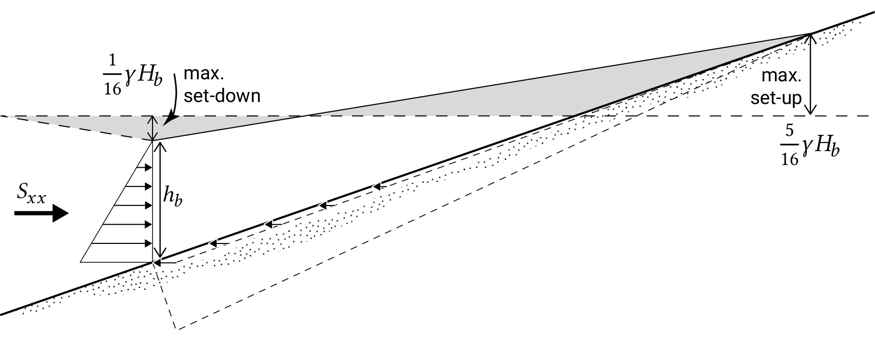
Note that the formulations for maximum set-down and set-up, shown in this figure, are analytically determined for normally incident waves and under the assumption of shallow water (pages 216-218 of the textbook).
Following week 1.5 of the MUDE and the first Wave Computer Lab, Eq. (1) can be discretized using forward Euler. This leads to:
\[\begin{equation} \tag{2a} F_{x,i} = - \frac{S_{xx,i+1}-S_{xx,i}}{x_{i+1}-x_{i}} \end{equation}\]
\[\begin{equation} \tag{2b} \overline{\eta}_{i+1}=\overline{\eta}_{i} - \frac{S_{xx,i+1}-S_{xx,i}}{\rho g h_i} \end{equation}\]
For an alonghore uniform coast, the alongshore wave force \(F_y\) is determined by the cross-shore gradient of the radiation shear stress \(S_{yx}\), with \(S_{yx}\) given by Eq. (5.53c) in the textbook. This wave force is balanced by a pressure force due to a water level gradient (see also Eq. (5.72) in the textbook):
\[\begin{equation} \tag{3} F_y = - \frac{dS_{yx}}{dx} = \overline{\tau}_{b,y} \end{equation}\]
and using forward Euler:
\[\begin{equation} \tag{4} F_{y,i} = - \frac{S_{yx,i+1}-S_{yx,i}}{x_{i+1}-x_{i}} \end{equation}\]
To compute the longshore current velocity, you can use Eq. (5.82) in the textbook and approximate \(h\) again as \(h_0\) (the mean water depth without wave-induced water level variations \(\overline{\eta}\)). You will also be asked to compute the near-bed orbital velocity amplitude according to linear wave theory, see Eq. (5.27) in the textbook.
How to use the results of Part 1 as a starting point?
Let’s first determine the input for the computations of Part 2. You have the following options in the below code cell: 1. If your function wave_transformation was correct, choose in the below code cell: “wave_transformation_function = True” and select input values. By running the cell the wave parameters L, c, n, cg, theta, Ksh, Kr, H and E are computed from your function wave_transformation with the chosen input values as input. 2. If your function wave_transformation was incorrect, choose in the below code cell: “wave_transformation_function = False”. By now running the cell, the wave parameters L, c, n, cg, theta, Ksh, Kr, H and E are loaded from file and the corresponding input values are assigned (do not change these; they correspond to the pre-calculated values).
Input at offshore boundary
Note that in Part 1, it was not necessary for the wave conditions at the offshore boundary to represent deep water. In this Part 2, this is different, since the solution to Eq. (2b) requires that \(\overline{\eta} = 0\) at the offshore boundary. Therefore, if you choose “wave_transformation_function = True”, you now have to make sure the input parameters (the ones you choose in the below cell for your offshore boundary conditions) represent deep water. If you choose “wave_transformation_function = False”, the input parameters are fixed (we have chosen them such that they represent deep water).
# Choose whether to load pre-calculated values or to continue with your above defined function wave_transformation
wave_transformation_function = False

if wave_transformation_function:
    # Choose the input values. Make sure / verify the offshore boundary is now in deep water.
    # (since we will assume that the set-down is zero at the offshore boundary)
    input_values = {
        "H_off": 2.0,             # offshore wave height [m]
        "T": 5,                   # wave period [s]
        "h_off": 25,              # water depth at offshore boundary [m]
        "slope": 1 / 100,         # bed profile slope [-]
        "rho": 1025,              # water density [kg/m^3]
        "theta_off": 30,          # wave angle at offshore boundary [degrees]
        "gamma": 0.8,             # wave breaking parameter [-]
    }
    # Do not change these lines:
    H_off, T, h_off, slope, rho, theta_off, gamma = input_values.values()
    L, c, n, cg, theta, Ksh, Kr, H, E = wave_transformation(H_off, T, h_off, slope, rho, theta_off, gamma)
else:
    # Do not change:
    fp_L = "../database/3_tides_nonlinearity/L_values.txt"
    fp_c = "../database/3_tides_nonlinearity/c_values.txt"
    fp_n = "../database/3_tides_nonlinearity/n_values.txt"
    fp_cg = "../database/3_tides_nonlinearity/cg_values.txt"
    fp_angle = "../database/3_tides_nonlinearity/θ_values.txt"
    fp_Ksh = "../database/3_tides_nonlinearity/Ksh_values.txt"
    fp_Kr = "../database/3_tides_nonlinearity/Kr_values.txt"
    fp_H = "../database/3_tides_nonlinearity/H_values.txt"
    fp_E = "../database/3_tides_nonlinearity/E_values.txt"

    L = np.loadtxt(fp_L)
    c = np.loadtxt(fp_c)
    n = np.loadtxt(fp_n)
    cg = np.loadtxt(fp_cg)
    theta = np.loadtxt(fp_angle)
    Ksh = np.loadtxt(fp_Ksh)
    Kr = np.loadtxt(fp_Kr)
    H = np.loadtxt(fp_H)
    E = np.loadtxt(fp_E)

    # Do not change these input values, they correspond to the pre-computed wave transformation parameters!
    input_values = {
        "H_off": 2.0,             # offshore wave height [m]
        "T": 5,                   # wave period [s]
        "h_off": 25,              # water depth at offshore boundary [m]
        "slope": 1 / 100,         # bed profile slope [-]
        "rho": 1025,              # water density [kg/m^3]
        "theta_off": 30,          # wave angle at offshore boundary [degrees]
        "gamma": 0.8,             # wave breaking parameter [-]
    }

print(input_values)
{'H_off': 2.0, 'T': 5, 'h_off': 25, 'slope': 0.01, 'rho': 1025, 'theta_off': 30, 'gamma': 0.8}Coding exercise: radiation stresses, wave forces and effects on mean water level and flow
In the below code cell, add code to the function radiation_stresses to compute: - Near-bed orbital velocity amplitude u0 (m/s) - Radiation normal stress Sxx (N/m) - Wave force Fx (N/m²) - Mean water level variation (set-down and set-up) η (m) - Radiation shear stress Syx (N/m) - Wave force Fy (N/m²) - Longshore current velocity V (m/s)
When you run the below cell, your variables will be compared with and plotted against the correct variables. If you leave the code cell unchanged, your answers will be assumed to be zero by default.
Note that the above-defined input values and values for L, c, n, cg, theta, Ksh, Kr, H, E are available in the function radiation_stresses. As the first line in the below code cell, an extra input parameter is appended: the friction coefficient to be used in Eq. (5.82) in the textbook.
# Add a value of cf to the input_values dictionary
input_values["cf"] = 0.01     # friction coefficient for the alongshore velocity [-]

def radiation_stresses(input_values, L, c, n, cg, theta, Ksh, Kr, H, E):

    H_off, T, h_off, slope, rho, theta_off, gamma, cf = input_values.values()

    h, x,*_ = mod_3c.depth_xrange(slope, h_off)

    g = 9.81

    """Complete the code here for the following parameters for each cross-shore location"""
    """Write your variables in terms of h, H_off, T, h_off, slope, rho, theta_off, gamma, cf"""
    """And in terms of  L, c, n, cg, theta, Ksh, Kr, H, E (for as far needed)"""

    u0 = None
    Sxx = None
    Fx = None
    eta = None

    Syx = None
    Fy = None
    V = None


    return Sxx, Fx, eta, Syx, Fy, V, u0

output, figure = mod_3c.check_radiation_stresses(input_values, L, c, n, cg, theta, Ksh, Kr, H, E, [radiation_stresses])
print(output)
display(figure)
Your function is:
Values for Sxx are incorrect.
Values for Fx are incorrect.
Values for η are incorrect.
Values for Syx are incorrect.
Values for Fy are incorrect.
Values for V are incorrect.
Summarizing figure
Now that you have computed the radiation stresses, wave forces, wave-induced water level variation and longshore current, we summarize these in a figure that may help you reflect on the results. The figure gives the cross-shore distribution of several wave characteristics for two different wave conditions that you can change using the wave conditions. Note again, that the computation of \(\overline{\eta}\) assumes \(\overline{\eta} = 0\) at the offshore boundary. You can use this figure to answer the reflective questions below.
app = mod_3c.pop_radiation_stresses()

(app)
Reflective questions
Run the next cell for seven multiple-selection questions, which you can answer using the summarizing figure(s). With each question, try to also think of the why behind it.
q = [
    "Q3c-angle-part2",
    "Q3c-fx-fy",
    "Q3c-breaking_wave_height-part2",
    "Q3c-slope-part2",
    "Q3c-longshoretransport",
    "Q3c-cross_shoretransport1",
    "Q3c-cross_shoretransport2"
]

question_industry.serve(q)
The end
You have reached the end of Notebook 3c. This was the last notebook of this week.