from pathlib import Path

import numpy as np
import pandas as pd
import hvplot.pandas
import holoviews as hv
import panel as pn
from bokeh.models.formatters import PrintfTickFormatter

import coastal_dynamics as cd
8d: Interventions and natural changes
You have reached the fourth and final notebook of week 8, which considers changes in the dynamic equilibrium of basins, due to interventions and natural changes. We are going to bring together many of the concepts covered in Chapter 9 to examine how natural changes and human interventions (like closing off part of the basin with a storm surge barrier) modify the morphology of tidal basins and their surrounding coastal systems. When a change occurs, the system may shift to a new equilibrium, which may result in a supply or demand of sediment. When the basin demands sediment, we talk about “sand hunger” or, in Dutch, “zandhonger”). The relative supply or demand will determine the impact on the rest of the coastal system. The most important concept is to be able to estimate how the relative supply or demand changes as the tidal prism, channels, and ebb-tidal delta change. These components are dynamically coupled in a sediment-sharing system.
This notebook contains 1 coding exercise and thirteen multiple-choice and multiple-selection questions. It consists of the following parts: 1. Equilibrium relationships for channels and ebb-tidal delta 2. Closures 3. Land reclamation 4. Relative sea level rise
Before starting this notebook, make sure you followed the lectures on Chapter 9 (or read the slides) and read Section 9.8 of the Coastal Dynamics Open Textbook, which is on changes in dynamic equilibrium.
First import some necessary packages
Let’s first import the libraries that we use for our analysis by running the next cells.
import sys

sys.path.append('../')

from modules import mod_8, mod_css

# Activate Panel and apply custom CSS
pn.extension(raw_css=mod_css.custom_css())
# read questions locally
questions = cd.read_questions(Path("../hashed_questions/8_tidal_basins_hashed.json"))
question_industry = cd.QuestionIndustry(questions)
cd.UseAnswersApp("Q8d").serve()Part 1: Equilibrium relationships
The general form of equilibrium relationships for the volume \(V\) of systems elements, based on the tidal prism \(P\), is:
\[\begin{equation} \tag{1} V_{eq} = C P^{n} \end{equation}\]
where \(n\) [-] is the power of the relationship and \(C\) is a coefficient with units m\(^{3-3n}\).
The volume of sand stored in the outer (ebb-tidal) delta has empirically been related to the tidal prism, as you can see in Eq. 9.3 in the book. According to this equation the (deposited sand) volume of the outer (ebb-tidal) delta is given by:
\[\begin{equation} \tag{2} V_{od} = C_{od} P^{1.23} \end{equation}\]
where \(C_{od}\) is an empirical coefficient, for which we will use \(C_{od} = 65.7 \cdot 10^{-4}\) m\(^{-0.69}\).
In the case that the flood-tidal delta spans the entire basin, an empirical relationship for the total basin channel volume is given by Eq. 9.17 in the book. According to this equation, the (water) volume of the channels below mean sea level (MSL) is given by:
\[\begin{equation} \tag{3} V_{c} = C_{v} P^{1.5} \end{equation}\]
where \(C_{v}\) is an empirical coefficient (\(65 \cdot 10^{-6}\) m\(^{-1.5}\) for the Wadden Sea, \(73 \cdot 10^{-6}\) to \(80 \cdot 10^{-6}\) m\(^{-1.5}\) for the Eastern Scheldt and (former) Grevelingen estuaries, as per Eysink (1991)). We will use the value \(C_{v} = 65 \cdot 10^{-6}\) m\(^{-1.5}\) in this notebook.
Plot the equilibrium relationships
Before we explore changes to the system, let’s first plot the volume of the channels and outer delta versus the tidal prism according to Eqs. 2 and 3. The plot created by the below code cell is the basis of Figures 9.35 and 9.36 from the book and, consequently, of the explorations in this notebook. The code creates an app that allows you to vary axes type (linear and log-log ), plotting range, coefficients and power.
The app may become unresponsive after running the cells in Part 2. If this happens, please relaunch the app or rerun the cell that generates the app.
(mod_8.intermezzo_app())Reflection on equilibrium relationships
Using the app, test the sensitivity of the various parameters and plot settings. While doing so try to answer the following questions: - Why do we show this as a log-log plot? What details can you see when you plot it with a linear scale? - What do the units of the coefficients depend on? - What happens when you adjust the coefficient or power? In the log-log plot, which one controls the slope of the lines and which one the intercept with the axes?
Now let’s connect this to the underlying physical concepts. Answer the questions below.
q = [
    "Q8d-sensitivity_tidal_prism",
    "Q8d-physics_Cod",
]

question_industry.serve(q)
Part 2: Closures
Now we are ready to explore the effects of the closure of part of a tidal basin by a dam. A real-life example is the closure of the Lauwerszee in 1969. We will neglect the role of the flats, and assume they are already more or less in equilibrium after the closure. Figure 9.35 shows the effect of two different closures (Closure 1 and Closure 2) on the volume of the channels below MSL and the ebb-tidal delta volume. We are going to try to reproduce these two interventions.
Closure 1 (Small \(\Delta V_c\)):
The closure of part of a tidal basin will result in a reduction of the tidal prism and channel volume. For closure 1 the numbers are (compare Table 9.6 in the book):
| Parameter | Value [10\(^6\) m\(^3\)] |
|---|---|
| Prism before | 600 |
| Prism after | 300 |
| Reduction \(\Delta V_c\) | 300 |
Note that \(\Delta V_c\) is the channel volume inside the area that was closed off (\(V\)ch, closure in the figure below). As such, positive values of \(\Delta V_c\) correspond to a reduction in the total channel volume. This convention will be important for later questions also.
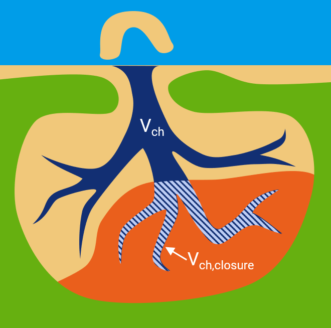
Coding exercise
Complete the code below to calculate \(V_{od}\) and \(V_c\) before and after Closure 1. Then, calculate the sediment demand of the channel \(a\) and the surplus of sand in the outer delta \(b\), so that we can interpret the consequences of the closure for the rest of the system. Use values of \(65.7 \times 10^{-4}\) and \(65 \times 10^{-6}\) for \(C_{od}\) and \(C_V\) respectively. In the code, replace the values of zero for \(V_c\), before, \(V_c\), after, \(V_{od}\), before, \(V_{od}\), after, \(a\), and \(b\) with the correct formulations. By running the code cells after, python will print and plot your answers and the correct answers (also compare these with the left plot of Figure 9.35 and the values in Table 9.6).
################# ADD CODE HERE ####################

V_c_before  = 0
V_c_after   = 0

V_od_before = 0
V_od_after  = 0

a = 0
b = 0

####################################################
mod_8.intervention(V_c_before, V_od_before, V_c_after, V_od_after, a, b, 0)| Parameter | Correct [10⁶ m³] | Student [10⁶ m³] | |
|---|---|---|---|
| 0 | Prism before | 600 | 600 |
| 1 | Prism after | 300 | 300 |
| 2 | Channel reduction ΔVᶜ | 300 | 300 |
| 3 | Vᶜ before | 955 | 0 |
| 4 | Vᶜ after | 337 | 0 |
| 5 | Demand of channels a | 317 | 0 |
| 6 | Vᵒᵈ before | 411 | 0 |
| 7 | Vᵒᵈ after | 175 | 0 |
| 8 | Surplus of outer delta b | 236 | 0 |
| 9 | Demand from outside a-b | 81 | 0 |
The following parameters are incorrect:
 V_c_before
 V_c_after
 V_od_before
 V_od_after
 a
 b

Have you included the 10^6 in your definition of P and V?
Questions about Closure 1 (small \(\Delta V_c\))
Did you get correct values for \(V_c\), before, \(V_c\), after, \(V_{od}\), before, \(V_{od}\), after, \(a\), and \(b\)? If not, you might have forgotten to include the 10\(^6\) in your values. Always remember to look at the units!
Now, using the plots generated above, answer the following reflective questions.
q = [
    "Q8d-outer_delta1",
    "Q8d-channels1",
    "Q8d-demand_and_supply1",
    "Q8d-long_term_evolution1",
]

question_industry.serve(q)
Closure 2 (large \(\Delta V_c\)):
Now let’s consider Closure 2 from the book (Figure 9.35 right plot), which assumes the same reduction in tidal prism but a relatively large reduction in channel volume (\(\Delta V_c\)). The values are given in the table below (see also Table 9.6).
| Parameter | Value [10\(^6\) m\(^3\)] |
|---|---|
| Prism before | 600 |
| Prism after | 300 |
| Reduction \(\Delta V_c\) | 470 |
We don’t require you to code again. Instead, run the cell below the generate an app in which you can change the tidal prism and channel volume reduction due to the closure. You can use this to consider the effect of different types of interventions.
(mod_8.fig935_app())WARNING:param.main: DataTabulator was not imported on instantiation and may not render in a notebook. Restart the notebook kernel and ensure you load it as part of the extension using:
pn.extension('tabulator')
Questions about Closure 2
Using the app, answer the following reflective questions.
q = [
    "Q8d-outer_delta_and_channels2",
    "Q8d-long_term_evolution2",
    "Q8d-tidal_signal_closure2",
]

question_industry.serve(q)
Part 2: Land reclamation
We can use the app to explore other interventions too. Let us consider a land reclamation, in which tidal flats are diked off and converted to usable land. As a consequence of this intervention, the tidal prism \(P\) reduces, but we do not reduce the volume of the channels \(V_c\) (as we are only reclaiming the tidal flats).
This land reclamation scenario differs from the “Accretion of New Land” scenario outlined in Chapter 9.8.2 mainly in terms of the relative timescales. The land reclamation is assumed to happen on the timescale of an engineering project (i.e., a few years), whereas the accretion of new land is something that may take decades or centuries. As such, the reduction of the tidal prism is more gradual and the system has more time to adjust.
The table below provides the numbers for the land reclamation scenario. Enter the numbers in the app to produce a figure.
| Parameter | Value [10\(^6\) m\(^3\)] |
|---|---|
| Prism before | 500 |
| Prism after | 250 |
| \(\Delta V_c\) | 0 |
Questions about land reclamation
Using the generated plot, answer the questions below.
q = [
    "Q8d-outer_delta_and_channels",
    "Q8d-adjacent_coast",
]

question_industry.serve(q)
Part 3: Relative sea level rise
Finally, we consider relative sea level rise. Understanding how tidal basins and estuaries will respond to rising sea levels (whether due to global sea level rise or local factors like subsidence) is a problem of critical importance to tomorrow’s coastal engineers (i.e., you!). For this exercise, we consider the values in the table below:
| Parameter | Value [10\(^6\) m\(^3\)] |
|---|---|
| Prism before | 750 |
| Prism after | 750 |
| Reduction \(\Delta V_c\) | -200 |
Note that here the tidal prism remains constant throughout the period under consideration. Why would that be? We will come back to this in the questions below. Further note that there is a negative reduction in channel volume (\(\Delta V_c\)). In other words, the channel volume increases in magnitude (recall the previous definition of \(\Delta V_c\) as the volume of channels removed by a closure being a positive value).
Again, use the app to explore this scenario.
Questions about relative sea level rise
Finally, answer the questions below.
q = [
    "Q8d-tidal_prism_with_SLR",
    "Q8d-wrapup",
]

question_industry.serve(q)
Reflection
As we have now seen, sea level rise and coastal interventions can lead to a demand for sediment (“sand hunger” or “zandhonger”), which is often met by the adjacent coasts. This is something that we can see from past interventions in the Dutch coastal system (e.g., the construction of the Delta Works). Our ability to meet this sediment demand in the decades ahead presents both technical challenges (do we have the right supply of sediment offshore to nourish the coast? how do we ensure that sediment gets to the places it needs to go? can we design interventions to minimize this sediment demand? how can we minimize negative ecological impacts from this approach?) and big societal questions (until which point are we willing to pay to maintain this sediment supply?) that will need to be answered by the coastal engineers of tomorrow (that’s you!).
The end
You have reached the end of this Notebook 8d: Interventions. Coincidentally, this also means you have reached the end of the final notebook of the course! We hope you have found value in these notebooks, and we would love to hear your feedback so we can improve the experience for future students and coastal engineers alike. Also, we hope to see you next quarter in the coastal module (and if not, good luck with your future studies)!