from pathlib import Path

import holoviews as hv
import hvplot.pandas  # noqa: API import
import numpy as np
import pandas as pd
import panel as pn

import coastal_dynamics as cd
6: Cross-shore transport
Welcome to this notebook on cross-shore sediment transport, which is the only notebook of week 6. The main topic of this notebook is cross-shore sediment transport (Chapter 7 of the Coastal Dynamics Open Textbook, with some extra attention for section 7.5 specifically). The notebook consists of three parts with a total of twenty-two questions.
- We will start with a recap of velocity moments as a proxy for sediment transport, including a more detailed look into Figure 7.21 from the book. This figure uses velocity moments to distinguish between the transport contributions by mean currents, long waves and short waves in typical storm conditions. We conclude this part with seven multiple-choice / - selection questions.
- Next, we will introduce the concept of shape functions for cross-shore transport, which will allow us to visualize cross-shore transport for different conditions. Herewith, we can draw conclusions about the differences between storm conditions and calmer conditions. This part contains fifteen multiple-choice / -selection questions to assist with interpretation.
- The optional third part suggests some additional topics to explore using the same visualizations as used in part 2. Even though it is slightly beyond the scope of Coastal Systems, it may help you to better understand cross-shore transport mechanisms. It may especially be nice if you think you may choose the Coastal B module, where we will get back to it.
We hope you have fun!
Import the required packages and questions
Run the below cells to import all necessary packages and question files required in this notebook.
import sys

sys.path.append('../')

from modules import mod_6, mod_css

# Activate Panel and apply custom CSS
pn.extension(raw_css=mod_css.custom_css())
# Use this cell to load questions
questions = cd.read_questions(Path("../hashed_questions/6_cross_shore_transport_hashed.json"))
question_industry = cd.QuestionIndustry(questions)
cd.UseAnswersApp("Q6").serve()Part 1: Velocity moments as a proxy for sediment transport
Theory
Remember from Chapter 5 that the velocity \(u\) close to the bed can be assumed to consist of a wave group-averaged component \(\bar{u}\), a short-wave-averaged oscillatory component \(u_{lo}\) and a short-wave oscillatory component \(u_{hi}\): \[ u = \bar{u} + u_{lo} + u_{hi} \] We are interested in the time-averaged sediment transport. We have used the third odd velocity moment as a proxy for the bed load transport and the fourth odd velocity moment as a proxy for suspended load transport. If \(\bar{u} \ll u_{lo} \ll u_{hi}\), the three most important terms in the third odd velocity moment are: \[ \left\langle u \left|u\right|^2\right\rangle = 3 \left\langle \bar{u} \left|u_{hi}\right|^2\right\rangle + \left\langle u_{hi} \left|u_{hi}\right|^2\right\rangle + 3 \left\langle u_{lo} \left|u_{hi}\right|^2\right\rangle + ... \]
Each of these terms is fully explained in the book, but in short, these terms refer to the following processes:
- \(3 \langle \bar{u} |u_{hi}|^2 \rangle\): transport of sediment stirred up by short waves and transported by the mean current
- \(\langle u_{hi} |u_{hi}|^2 \rangle\): transport of sediment stirred up by short waves and transported by the high-frequency waves
- \(3 \langle u_{lo} |u_{hi}|^2 \rangle\): transport of sediment stirred up by short waves and transported by the low-frequency waves
Each of the velocity moments can be directly measured in a flume or computed, or a combination of the two, which is what Roelvink and Stive (1989) did to obtain the results of Figure 7.21 in the book. In quite some quasi-steady sediment transport formulations, one can recognize the velocity moments. For instance, have a look at Eqs. 6.48a and 6.48b in the textbook.
There will be a net transport along the profile if the profile is not in equilibrium with the conditions. This is for instance the case when a profile built up by smaller waves is suddenly under the influence of larger storm waves. These larger storm waves will redistribute the sediment to a flatter, post-storm profile. The other way around also holds true: it is possible to mathematically derive an equilibrium profile by balancing the onshore and offshore terms. Bowen (1980) does this analytically for the middle and lower shoreface by equating onshore transport by short waves with offshore transport by gravity.
Figure 7.21
Now have a look at Figure 7.21 from the book (below). As mentioned before, we use the velocity moments as a proxy for sediment transport. The total transport can then be decomposed into multiple gross contributions by decomposition of the velocity moments. For instance, the upper panel of Figure 7.21 gives the total third odd moment as well its three components given by the right-hand side of the above equation. Note that the onshore direction is defined as the positive x-direction, and that, therefore, velocities and transports are positive in onshore direction, and negative in offshore direction.
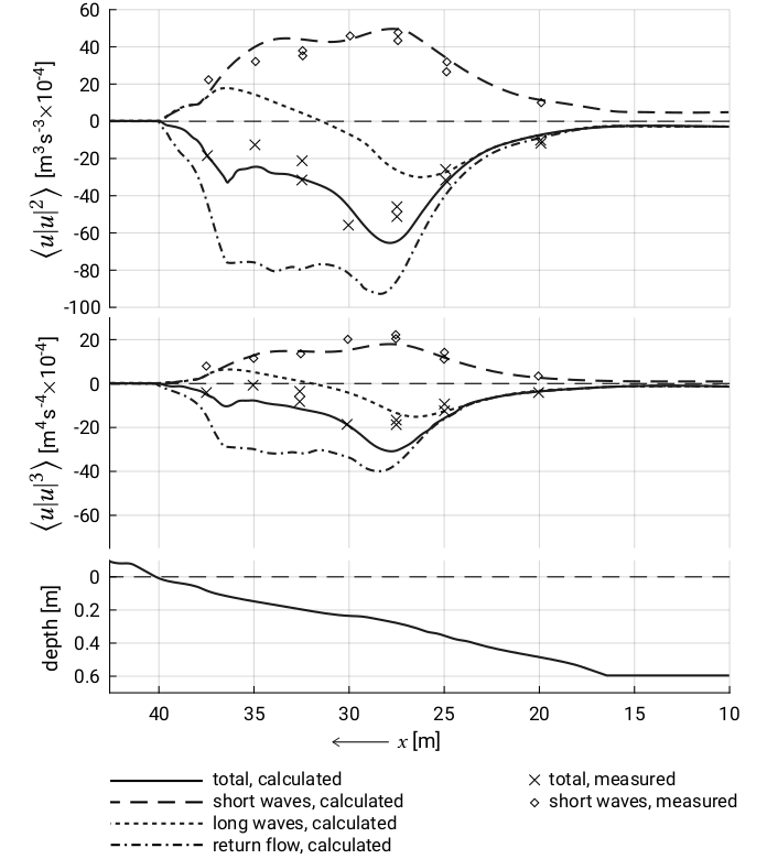
Questions about Figure 7.21
Run the cell below to get seven questions about Figure 7.21.
q = [
    "Q6-direction_total",
    "Q6-direction_mean",
    "Q6-direction_skewness",
    "Q6-direction_long",
    "Q6-breakpoint_position",
    "Q6-conditions_fig721",
    "Q6-morphological_response",
]

question_industry.serve(q)
Part 2: Shape functions for cross-shore transport
Wouldn’t it be nice to know how Figure 7.21 would change for different wave conditions and bathymetry? However, we are limited by the lack of direct observations. Tinker et al. (2009) present a solution. They performed a large number of suspended transport measurements close to the bed (in the bottom 15 cm) and fitted a shape function for transport due to both mean and oscillatory flow in the surf/shoaling zone (Figure 5 in their paper). In this Part 2, we will focus on this mean and oscillatory flux in the surf/shoaling zone and compare this with Figure 7.21.
Tinker et al. (2009) differentiate between transport in the surf/shoaling zone, and the swash/(inner) surf zone. As in Figure 7.21, they define transport as positive in the onshore direction. Transport in the surf/shoaling zone was separated in a mean and oscillatory transport (or flux), and transport in the swash/surf zone in an onshore and offshore component. This means that in the surf/shoaling zone, both high- and low-frequency waves are combined in the ‘oscillatory’ component. In part I, we already discussed the concept of mean transport (as a result of undertow) and oscillatory transport (resulting from high- and low-frequency waves) in the shoaling and surf zone. The main difference now with Figure 7.21 from the book is that long and short waves are not considered separately by Tinker et al.
It is important to note that these shape functions represent suspended sediment transport only. Measurements were made at various heights above the bed (in the bottom 15 cm). The measurements by Tinker et al. were done at Sennen Cove, Cornwall, UK. For some context, the mean spring tidal range (MSTR) at this site is 5.3 m, which makes this a macrotidal system. The average significant wave height is 1.4 m, and the median grain size is 0.7 mm. This is quite coarse sediment (when compared to for instance the Dutch coast), so we can expect quite a steep bed profile. This bed profile is discussed further below.
In addition, Tinker et al. measured and determined shape functions for onshore and offshore transport in the swash/inner surf zone. The swash zone is the region at the shoreline where waves wash up and down the beach face. The transport in the swash zone can be quite important, but it is not easy to model and it is therefore not always taken into account in models. The study of Roelvink and Stive (Figure 7.21) did not take the swash zone into account, either. Later, in Part 3, you will have the opportunity to look at the swash/inner surf zone transport. Though the paper is very interesting (and we definitely recommend checking it out), you are not required to know it for this exercise or for Coastal Systems (CIEM3110). Details about swash transport are also outside the scope of Coastal Systems. You will hear more about this paper and these concepts in the Coastal module (CIEM3210), if you choose it!
Prepare the visualization
By executing the below cells we are now going to prepare the visualization in a couple of steps: 1. Define the shape functions for the transport 2. Define the bathymetry functions 3. Plot the results
Define the shape functions for the transport
Below the shape functions as presented by Tinker et al. (2009) are defined.
Note: You are not expected to know or remember these equations, they are just here to help us with the exercise. Nonetheless, it is useful to understand what the most important variables are in the shape functions. To that end, scroll through the code of the below cell before executing it.
You should find that for the surf/shoaling zone, the shape functions depend on the local water depth \(h\) and on the water depth at breaking \(h_b\). The larger that \(h_b\) is, the more energetic that the waves are. Remember that in notebook 3c you have determined \(h_b\) as part of the calculation of the cross-shore distribution of the wave heights in the shoaling zone and surf zone. Note that this parameterization ignores the presence of infragravity (i.e., bound or free long) waves.
### Shape functions for the surf/shoal zone ###

# mean transport
def Tinker_mean(h, h_b):
    tp = (-120 * h_b**2) * (h / h_b)**4.3 * np.exp(-9.4 * (h / h_b)**0.75)
    return tp

# oscillatory transport
def Tinker_osci(h, h_b):
    tp = (2.75 * h_b**0.6) * (h / h_b)**3.5 * np.exp(-4.2 * (h / h_b)**1.05)
    return tp

# surf / shoal zone (mean + oscillatory transport)
def Tinker_surf_shoal(h, h_b):
    tp = Tinker_mean(h, h_b) + Tinker_osci(h, h_b)
    return tp

### Shape functions for the swash/surf zone ###

# onshore transport
def Tinker_onsh(h, h_b):
    tp = 3.5 * h_b**1.9 * (h / h_b)**1.1 * np.exp(-31 * (h / h_b)**1.1)**(h_b**1.1)
    return tp

# offshore transport
def Tinker_offs(h, h_b):

    con1 = (h_b > 2.15)
    con2 = (h_b <= 0.75)
    con3 = ((h_b <= 2.15) * (h_b > 0.75))

    a_off = \
        con1 * (-3 * h_b + 4) + \
        con2 * 0 + \
        con3 * (-1.25 * (h_b - 0.75)**2)

    tp = a_off * h_b**1.1 * (h / h_b)**1.1 * np.exp(-5.7 * (h/h_b)**1.1)**(h_b**1.1)
    return tp

# swash / surf zone (onshore + offshore transport)
def Tinker_swash_surf(h, h_b):
    tp = Tinker_onsh(h, h_b) + Tinker_offs(h, h_b)
    return tp

### Total transport for swash/surf/shoal ###

# total transport (mean + oscillatory + onshore + offshore transport)
def Tinker_total(h, h_b):
    tp = Tinker_surf_shoal(h, h_b) + Tinker_swash_surf(h, h_b)
    return tp

Tinker_functions = (
    Tinker_mean,
    Tinker_osci,
    Tinker_surf_shoal,
    Tinker_onsh,
    Tinker_offs,
    Tinker_swash_surf,
    Tinker_total,
)
Define bathymetry functions
The functions in the cell below define the bathymetry. Two different bathymetries are defined. The first is used by Tinker et al. (2009) to define their shape functions. As mentioned, this is the bathymetry at Sennen Cove, Cornwall, UK. The second bathymetry is the bathymetry shown in Figure 7.21 in the textbook. Roelvink and Stive (1989) used this bathymetry for small-scale flume experiments performed at Delft Hydraulics (now Deltares). We will also use parabolic profiles, as in Figure 7.8 in the textbook. They will be defined in the plot function. The onshore direction is defined as the positive x-direction.
# Bathymetries here!

# define paths
fp_uk = Path("../database/6_cross_shore_transport/6_uk_bath.csv")
fp_nl = Path("../database/6_cross_shore_transport/6_nl_bath.csv")

# read bathymetry files
df_uk = pd.read_csv(fp_uk, sep='; ', decimal=',', names=['x', 'y'], engine='python')
df_nl = pd.read_csv(fp_nl, sep='; ', decimal=',', names=['x', 'y'], engine='python')

# interpolate to suitable grid
uk_bath = mod_6.interpolate_bathymetry(fp_uk)
nl_bath = mod_6.interpolate_bathymetry(fp_nl)

baths = {
    "Sennen Cove, Cornwall (UK)": uk_bath,
    "Scheldt flume (NL)": nl_bath,
}
Plot the results
The next cell calls the plot function. It plots the Tinker shape functions, which are a function of \(h/h_b\), and translates these to a function of the cross-shore distance \(x\) for a particular bathymetry.
In order to facilitate the analysis, the cross-transport gradients are also calculated and plotted as a function of \(x\). We compute the transport gradients \(dQ/dx\) in the direction of positive transports \(Q\), so in positive x-direction. This ensures that positive gradients imply an increasing transport and, hence, a negative bed change or erosion. This guarantees that for every location, we can interpret positive gradients as leading to erosion and negative gradients as leading to sedimentation.
Now we can plot the results! Execute the cell below to generate the plot by using the function we defined above.
app = mod_6.show_transport(baths, Tinker_functions)

(app)
The transport panel
You now have a panel with four plots: 1. Cross-shore profile (vertical distance above a reference as a function of the cross-shore position \(x\) 2. Transport as a function of the cross-shore position \(x\) - defined such that onshore transport is positive 3. Transport gradients \(dQ/dx\) as a function of cross-shore position \(x\) - defined such that positive gradients imply erosion 4. Tinker shape functions (transports as a function of \(h/h_b\) with \(h/h_b = 1\) the breakpoint)
The panel has the following options: 1. You can select the bathymetry you want to look at using the selector in the panel 2. You can use the sliders to change the water level and breaker depth (plotted as a horizontal dashed blue and a vertical grey line respectively) 3. When the parabolic profile is selected, it becomes relevant to adjust the A and m values to your liking (take another look at Chapter 7.2.2 of the textbook for more details on these parameters) 4. You can choose whether to include certain transport components in the transport plot or not. By default, only the mean transport and the oscillatory transport are included
Please note that the transport gradients in the plot are sometimes not entirely smooth; you can ignore these small-scale fluctuations.
Intermezzo: transport gradients
Understanding how sediment transport gradients lead to erosion or sedimentation (and how to visualize that or estimate it by looking at a figure) is a really important part of this course, so it is worth spending the time here to understand what is going on. This concept will come up again in other parts of the course (like alongshore transport). Verify for yourself that:
- A transport maximum or minimum implies a zero transport gradient and zero bed change;
- Where the transport changes fastest along the profile, the transport gradients have the largest magnitude and the bed changes are largest;
- A positive transport gradient implies erosion; this happens if the positive (onshore) transport increases in positive x-direction (onshore) or if the negative (offshore) transport increases in negative x-direction (offshore);
- A negative transport gradient implies accretion; this happens if the positive (onshore) transport decreases in positive x-direction (onshore) or if the negative (offshore) transport decreases in negative x-direction (offshore).
General questions about the transport panel
In this part 2, let’s stick to the default by only looking at mean and oscillatory transport in the surf/shoal zone. Also tick the box for total transport in the surf / shoal zone. Only in Part 3 does the swash/surf zone become relevant.
Execute the cell below for two general questions about the transport panel. When you answer the questions, do not only consider the transports along the profile, but the transport gradients as well.
q = [
    "Q6-unit_a",
    "Q6-unit_b",
]

question_industry.serve(q)
Questions about the transport in the surf/shoal zone of Sennen Cove for high-energy conditions
With our plotting function defined, let’s first look at the United Kingdom site where the measurements were made. Select “Sennen Cove, Cornwall (UK)” in the bathymetry selector.
The measurements were done over many tides (39) and for a range of wave conditions (offshore significant wave heights ranging from 0.1–2.5 m. Firstly, we will look at the more energetic conditions, which might occur during a storm. According to Tinker et al., a breaker depth of \(h_b=2\) m is representative of such a situation. Use this value.
For Sennen Cove, the reference level in the plot is mean sea level (MSL). Using the slider, you can set the water level relative to MSL, depending on the stage of the tide. First, play around with this slider. You should notice that for lower tidal water levels, not only the shoreline but also the breakpoint shifts in the offshore direction. This is a nice example of how the tide level affects which part of the profile is under wave attack. You should also notice that for MSL, the breakpoint is just outside the measured profile (and its instrumentation for the velocity and concentration measurements). It even falls outside the considered profile for lower tide levels. Clearly, the coverage of measurements in the shoaling zone depended on the tide and wave conditions. Under high-energy conditions data beyond the breakpoint were limited. We must keep this in mind when interpreting the shape functions.
Now set the water level to MSL +2 m (this is MHWS).
We are now going to look at the transports (second panel and fourth panel) and transport gradients (third panel) along the profile. Make sure to have selected the mean, oscillatory and total transport in the surf / shoal zone. Keep in mind that the horizontal axis in the second and third panels are the same as that of the profile. In the fourth panel, however, the transport is given as a function of \(h/h_b\) (with \(h/h_b = 1\) the breakpoint).
Execute the below cells to generate the questions, which will help you explore the transport in the surf/shoal zone of Sennen Cove for high-energy conditions.
q = [
    "Q6-width_surf_zone",
    "Q6-direction_waves_undertow",
    "Q6-onshore_transport_waves",
    "Q6-offshore_transport_undertow",
    "Q6-direction_total_high_energy",
    "Q6-compare_Tinker_book",
    "Q6-morphological_response_surf",
    "Q6-morphological_response_shoal",
]

question_industry.serve(q)
Questions about the transport in the surf/shoal zone of Sennen Cove for low-energy conditions
Before we explore the low-energy conditions, let’s summarize some of our findings for the high-energy conditions. We see an offshore mean transport due to undertow in the surf zone (and a little bit outside) and an onshore oscillatory transport in the shoaling zone and surf zone. This gives a total transport with an offshore maximum in the surf zone and an onshore maximum near the breakpoint (just outside the breakpoint). These maxima separate the regions of accretion and erosion, as you can verify from the plot of the transport gradients. The largest changes are in the surf zone, where sediment is moved from higher to lower portions of the profile. But sediment is also brought from the shoaling zone to the accretion zone in the outer part of the surf zone.
Now we continue with looking at low-energy conditions for Sennen Cove, which according to Tinker et al. is represented by a breaking depth \(h_b=0.6\) m. Change the value of \(h_b\) in the plot to 0.6 m. For ease of comparison, set the water level again to MSL +2 m (this is MHWS).
You can immediately see that for the low-energy conditions, the surf zone is very narrow. As a consequence, the instruments were not in the surf zone for a very long time, resulting in little data from this region. This introduces some uncertainty in the resulting shape functions.
Try to answer the questions below for the low-energy conditions.
q = [
    "Q6-width_surf_zone2",
    "Q6-transport_direction_waves_undertow",
    "Q6-difference_high_low_energy",
    "Q6-morphodynamic_response_transport_maximum",
]

question_industry.serve(q)
Concluding question for Sennen Cove exploration
By now, you have explored the main concepts of cross-shore sediment transport employing the shape functions by Tinker et al. The low-energy shape function can lead to the development of the typical summer/calm profile and drive onshore bar migration. The high-energy shape function can lead to the development of the typical winter/storm profile and drive offshore bar migration.
A key feature of the two shape functions is that both the mean and oscillatory sediment fluxes increase with \(h_b\), but that the offshore-directed mean flux increases faster than the onshore-directed oscillatory flux. For small \(h_b\), the net transport is onshore regardless of \(h/h_b\). For larger \(h_b\), the net transport has an offshore transport peak in the surf zone and an onshore transport peak close to the breakpoint. Use the \(h_b\) slider to verify these conclusions. When you have done so, try to answer the following question:
q = [
    "Q6-onshore_equals_offshore",
]

question_industry.serve(q)
Part 3: Optional Extra Material
If you are curious, you can optionally continue to explore some additional features that we built in this notebook.
(\(h / h_b\))-plot
As you will have noticed by now, the plotting function generates four subplots: the bathymetry, the transport and transport gradients as a function of \(x\), and the transport as a function of \(h/h_b\). The dimensionless \(h/h_b\) is a convenient way to normalize cross-shore profiles. Below, a new plotting method is defined to look at this manner of plotting more closely. You will see that this way of looking at it can help to better understand the above explored dependencies of the transport and morhological response on \(h_b\) and generalize the conclusions.
To that end, we will create a new panel, where the transport is plotted as a function of \(h/h_b\) for an (adjustable) range of values for \(h_b\). Using this panel, it is much easier to explore the effect of \(h_b\). We will not ask any specific questions about this plot. Instead, try to verify some of the key features of the shape functions. For this, you can have a look at the following pointers: - both the mean and oscillatory sediment fluxes increase with \(h_b\). - the offshore-directed mean flux increases faster than the onshore-directed oscillatory flux. - for small \(h_b\), the net transport is onshore regardless of \(h/h_b\). - for larger \(h_b\), the transport has an offshore transport peak in the surf zone and an onshore transport peak close to the breakpoint. - the onshore and offshore net transport peaks are approximately equal in magnitude for \(h_b\) = 1.7 m. - the low-energy shape function can lead to the development of the typical summer/calm profile and drive onshore bar migration. - the high-energy shape function can lead to the development of the typical winter/storm profile and drive offshore bar migration.
It is also nice to compare our (\(h / h_b\))-plot with Figs. 6 and 8 in Tinker et al. (2009).
Now execute the cell below to obtain the (\(h / h_b\))-plot. Make sure the total transport is also selected, then play around with the (\(h_b\))-slider and try to verify the pointers listed above.
app = mod_6.h_hb_transport(Tinker_functions)

(app)
Scheldt Flume
It is a nice additional exercise to now select the Scheldt Flume profile in the first panel and see how the shape functions behave for the situation as in Figure 7.21. Set the water level slider at the reference level and choose the \(h_b\), such that it gives you the surf zone width that you estimated in Q5 above. What do you learn from this comparison?
Because the Scheldt Flume is a small-scale facility and not at full size, the value for \(h_b\) is very small (≈ 0.35 m). In real life such a value for \(h_b\) would represent accretive conditions conditions and the shape functions do indeed give a consistent onshore transport. In the Scheldt Flume, however, these waves mimic storm conditions.
Intermezzo: Physical Scale Modelling of Sediment Transport
Physical modelling studies of sediment transport are extremely difficult due to the matter of scaling. When a beach is scaled down by a factor of 10-50 to be simulated in the lab, not everything scales linearly (e.g., the width of the beach does not shrink by the same proportion as do the forces exerted by waves on sand grains) and sediment properties change fundamentally. In spite of these challenges, scale models are often still “unreasonably effective” at elucidating physical processes, even when compromises in scaling have to be made.
Parabolic profile
The shape functions from Tinker et al. were developed for the Sennen Cove site (UK) with a \(D_{50}\) ≈ 0.7 mm (relatively coarse sand). Nonetheless, the authors assume that the shape functions are generally applicable to sandy beaches with alongshore uniform topography (although some adjustments must be made to make them work on a barred beach).
Let’s try the shape functions for different types of bathymetry, assuming some breakpoint depth \(h_b\)! For this, we have included the option for a parabolic coastal profile in the first panel. You can select the parabolic coastal profile using the dropdown menu in the plot and set the two parameters A and m using the sliders. In this way, you can study the difference between the three Dutch profiles of Figure 7.8 in the book and make a comparison to Sennen Cove.
Here are some observations that you can make: 1. For the three Dutch sites \(D_{50}\) ≈ 0.2 mm rather than \(D_{50}\) ≈ 0.7 mm. The grain-size, however, does not play a role in the shape functions and, consequently, for the same \(h_b\) the “predicted” seaward and shoreward transport maxima have the same magnitude for all four profiles. We can question whether it is realistic that the grain-size does not play a role. 2. Also the profile steepness varies between the profiles. All Dutch sites are significantly less steep than the UK site, and the Dutch sites also vary in steepness (check which is the steepest and which the flattest in Figure 7.8). 4. For the same \(h_b\), a steeper profile leads to a narrower zone in which the transport takes place. You can check this by choosing a value for \(h_b\) and considering the surf zone width and extension of the transport zones for all four profiles. 5. In the comparison, we started from the same value for \(h_b\). Note that the profile steepness also plays a role in the wave breaking and, hence, breaker index \(\gamma\) (see Section 5.2.5). Therefore, the wave height at breaking could vary between the profiles even if \(h_b\) is the same.
Please note that it is a bit inconsistent to look at instantaneous sediment transport on a parabolic equilibrium profile that is derived based on a long term average. It is always important to reflect on the assumptions behind the equations or models that you use to describe the coast before you apply them to a new setting!
Transport in the swash zone
Including the on- and offshore transport shape functions allows us to look at what happens in the swash and the inner surf zone. Enable these functions in the plot to explore the effect of including the transport in the swash / inner surf zone. You can use both the first panel and the second panel. The second panel probably gives the best overview for a range of \(h_b\)-values.
See if you can verify the following statements: 1. By definition, the onshore transport component of the swash /inner surf zone is always positive (i.e., in positive x-direction, which is defined as onshore), whereas the offshore transport component is always negative. 2. The onshore transport occurs under all conditions and is confined to very shallow water 3. The offshore component only occurs during high-energy conditions and takes place a bit further offshore in the inner surf zone (but still in the swash/inner surf zone). 4. During high-energy conditions, the offshore transport function helps explain rapid erosion in the outer swash/inner surf zone, by pulling the offshore transport maximum shorewards.
The end
You have reached the end of this notebook for week 6 (the only notebook of this week). You now know about the different components in the swash, surf, and shoaling zones under high-energy and low-energy conditions, and have seen some practical examples! In ACES (the first unit of the B1 Coastal Engineering module, CIEM3210) we will discuss the Tinker et al. paper further.